Hamilton–Jacobi equation
In mathematics, the Hamilton–Jacobi equation is a necessary condition describing extremal geometry in generalizations of problems from the calculus of variations. In physics, the Hamilton–Jacobi equation (HJE) is a reformulation of classical mechanics and, thus, equivalent to other formulations such as Newton's laws of motion, Lagrangian mechanics and Hamiltonian mechanics. The Hamilton–Jacobi equation is particularly useful in identifying conserved quantities for mechanical systems, which may be possible even when the mechanical problem itself cannot be solved completely.
The HJE is also the only formulation of mechanics in which the motion of a particle can be represented as a wave. In this sense, the HJE fulfilled a long-held goal of theoretical physics (dating at least to Johann Bernoulli in the 18th century) of finding an analogy between the propagation of light and the motion of a particle. The wave equation followed by mechanical systems is similar to, but not identical with, Schrödinger's equation, as described below; for this reason, the HJE is considered the "closest approach" of classical mechanics to quantum mechanics.[1][2]
Mathematical formulation
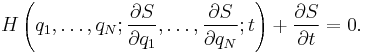
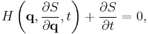
The Hamilton–Jacobi equation is a first-order, non-linear partial differential equation for a function  called Hamilton's principal function
As described below, this equation may be derived from Hamiltonian mechanics by treating  as the generating function for a canonical transformation of the classical Hamiltonian
  . The conjugate momenta correspond to the first derivatives of with respect to the generalized coordinates

As a solution to the Hamilton-Jacobi equation, the principal function contains N+1 undetermined constants, the first N of them denoted as  , and the last one coming from the integration of
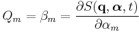
  . The relationship then between p and q describes the orbit in phase space in terms of these constants of motion. Furthermore, the quantities
are also constants of motion, and these equations can be inverted to find q as a function of all the  and
and  constants and time.[3]
Comparison with other formulations of mechanics
The HJE is a single, first-order partial differential equation for the function of the  generalized coordinates
  and the time
  . The generalized momenta do not appear, except as derivatives of . Remarkably, the function is equal to the classical action.
For comparison, in the equivalent Euler–Lagrange equations of motion of Lagrangian mechanics, the conjugate momenta also do not appear; however, those equations are a system of , generally second-order equations for the time evolution of the generalized coordinates. Similarly, Hamilton's equations of motion are another system of  first-order equations for the time evolution of the generalized coordinates and their conjugate momenta
  .
.
Since the HJE is an equivalent expression of an integral minimization problem such as Hamilton's principle, the HJE can be useful in other problems of the calculus of variations and, more generally, in other branches of mathematics and physics, such as dynamical systems, symplectic geometry and quantum chaos. For example, the Hamilton–Jacobi equations can be used to determine the geodesics on a Riemannian manifold, an important variational problem in Riemannian geometry.
Notation
For brevity, we use boldface variables such as  to represent the list of generalized coordinates
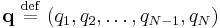
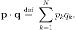
that need not transform like a vector under rotation. The dot product is defined here as the sum of the products of corresponding components, i.e.,
Derivation
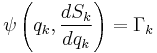
Any canonical transformation involving a type-2 generating function  leads to the relations
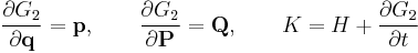
(See the canonical transformation article for more details.)
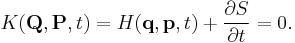
To derive the HJE, we choose a generating function  that makes the new Hamiltonian
  identically zero. Hence, all its derivatives are also zero, and Hamilton's equations become trivial
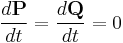
i.e., the new generalized coordinates and momenta are constants of motion. The new generalized momenta  are usually denoted , i.e.,
  .
.
The equation for the transformed Hamiltonian
Let
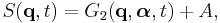
where A is an arbitrary constant, then S satisfies HJE
since  .
.
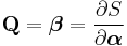
The new generalized coordinates  are also constants, typically denoted as
 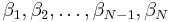 . Once we have solved for
  , these also give useful equations
or written in components for clarity
Ideally, these equations can be inverted to find the original generalized coordinates as a function of the constants  and
and  , thus solving the original problem.
Action
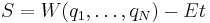
Both Hamilton principal function S and characteristic function are closely related to action.
The time derivative of S is
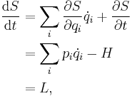
therefore
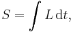
so S is actually classical action plus an undetermined constant.
When H does not explicitly depend on time,
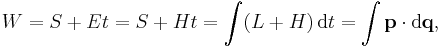
in this case W is the same as abbreviated action.
Separation of variables
The HJE is most useful when it can be solved via additive separation of variables, which directly identifies constants of motion. For example, the time can be separated if the Hamiltonian does not depend on time explicitly. In that case, the time derivative in the HJE must be a constant (usually denoted  ), giving the separated solution
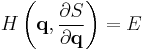
where the time-independent function  is sometimes called Hamilton's characteristic function. The reduced Hamilton–Jacobi equation can then be written
To illustrate separability for other variables, we assume that a certain generalized coordinate  and its derivative
  appear together in the Hamiltonian as a single function

In that case, the function can be partitioned into two functions, one that depends only on and another that depends only on the remaining generalized coordinates

Substitution of these formulae into the Hamilton–Jacobi equation shows that the function  must be a constant (denoted here as
  ), yielding a first-order ordinary differential equation for
In fortunate cases, the function can be separated completely into functions 

In such a case, the problem devolves to ordinary differential equations.
The separability of depends both on the Hamiltonian and on the choice of generalized coordinates. For orthogonal coordinates and Hamiltonians that have no time dependence and are quadratic in the generalized momenta, will be completely separable if the potential energy is additively separable in each coordinate, where the potential energy term for each coordinate is multiplied by the coordinate-dependent factor in the corresponding momentum term of the Hamiltonian (the Staeckel conditions). For illustration, several examples in orthogonal coordinates are worked in the next sections.
Example of spherical coordinates
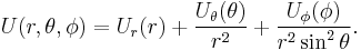
In spherical coordinates the Hamiltonian of a free particle moving in a conservative potential  can be written
![H = \frac{1}{2m} \left[ p_{r}^{2} %2B \frac{p_{\theta}^{2}}{r^{2}} %2B \frac{p_{\phi}^{2}}{r^{2} \sin^{2} \theta} \right] %2B U(r, \theta, \phi)](/2012-wikipedia_en_all_nopic_01_2012/I/f079ba61bf3870ed897d43041448f7d4.png)
The Hamilton–Jacobi equation is completely separable in these coordinates provided that there exist functions  ,
,  and
and  such that can be written in the analogous form
Substitution of the completely separated solution  into the HJE yields
![\frac{1}{2m} \left( \frac{dS_{r}}{dr} \right)^{2} %2B U_{r}(r) %2B
\frac{1}{2m r^{2}} \left[ \left( \frac{dS_{\theta}}{d\theta} \right)^{2} %2B 2m U_{\theta}(\theta) \right] %2B
\frac{1}{2m r^{2}\sin^{2}\theta} \left[ \left( \frac{dS_{\phi}}{d\phi} \right)^{2} %2B 2m U_{\phi}(\phi) \right] = E](/2012-wikipedia_en_all_nopic_01_2012/I/959c015479996d3485f8b524f915904c.png)
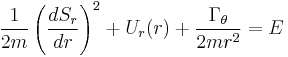
This equation may be solved by successive integrations of ordinary differential equations, beginning with the  equation
where  is a constant of the motion that eliminates the dependence from the Hamilton–Jacobi equation
![\frac{1}{2m} \left( \frac{dS_{r}}{dr} \right)^{2} %2B U_{r}(r) %2B
\frac{1}{2m r^{2}} \left[ \left( \frac{dS_{\theta}}{d\theta} \right)^{2} %2B 2m U_{\theta}(\theta) %2B \frac{\Gamma_{\phi}}{\sin^{2}\theta} \right] = E](/2012-wikipedia_en_all_nopic_01_2012/I/fcc06ea8d6e6c2ab08848e802f1f8f6f.png)
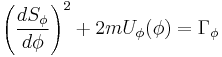
The next ordinary differential equation involves the  generalized coordinate
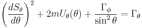
where  is again a constant of the motion that eliminates the dependence and reduces the HJE to the final ordinary differential equation
whose integration completes the solution for .
Example of elliptic cylindrical coordinates
The Hamiltonian in elliptic cylindrical coordinates can be written
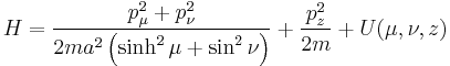
where the foci of the ellipses are located at  on the
  -axis. The Hamilton–Jacobi equation is completely separable in these coordinates provided that has an analogous form
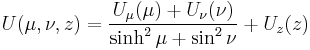
where  ,
,  and
and  are arbitrary functions. Substitution of the completely separated solution
  into the HJE yields
![\frac{1}{2m} \left( \frac{dS_{z}}{dz} \right)^{2} %2B U_{z}(z) %2B
\frac{1}{2ma^{2} \left( \sinh^{2} \mu %2B \sin^{2} \nu\right)} \left[ \left( \frac{dS_{\mu}}{d\mu} \right)^{2} %2B \left( \frac{dS_{\nu}}{d\nu} \right)^{2} %2B 2m a^{2} U_{\mu}(\mu) %2B 2m a^{2} U_{\nu}(\nu)\right] = E](/2012-wikipedia_en_all_nopic_01_2012/I/f1061558ca1b0ad6dae2b85b24806c72.png)
Separating the first ordinary differential equation
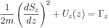
yields the reduced Hamilton–Jacobi equation (after re-arrangement and multiplication of both sides by the denominator)

which itself may be separated into two independent ordinary differential equations
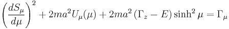
that, when solved, provide a complete solution for .
Example of parabolic cylindrical coordinates
The Hamiltonian in parabolic cylindrical coordinates can be written
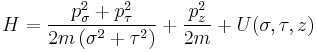
The Hamilton–Jacobi equation is completely separable in these coordinates provided that has an analogous form
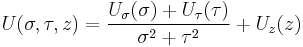
where  ,
,  and are arbitrary functions. Substitution of the completely separated solution
  into the HJE yields
![\frac{1}{2m} \left( \frac{dS_{z}}{dz} \right)^{2} %2B U_{z}(z) %2B
\frac{1}{2m \left( \sigma^{2} %2B \tau^{2} \right)} \left[ \left( \frac{dS_{\sigma}}{d\sigma} \right)^{2} %2B \left( \frac{dS_{\tau}}{d\tau} \right)^{2} %2B 2m U_{\sigma}(\sigma) %2B 2m U_{\tau}(\tau)\right] = E](/2012-wikipedia_en_all_nopic_01_2012/I/c67fbb3c9cb32e47f9822da97560ac33.png)
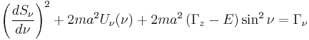
Separating the first ordinary differential equation
yields the reduced Hamilton–Jacobi equation (after re-arrangement and multiplication of both sides by the denominator)

which itself may be separated into two independent ordinary differential equations
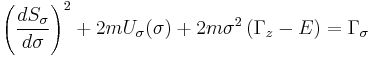
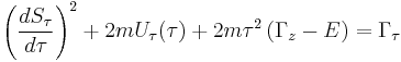
that, when solved, provide a complete solution for .
Eikonal approximation and relationship to the Schrödinger equation
The isosurfaces of the function  can be determined at any time . The motion of an -isosurface as a function of time is defined by the motions of the particles beginning at the points on the isosurface. The motion of such an isosurface can be thought of as a wave moving through space, although it does not obey the wave equation exactly. To show this, let represent the phase of a wave
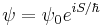
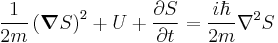
where  is a constant introduced to make the exponential argument unitless; changes in the amplitude of the wave can be represented by having be a complex number. We may then rewrite the Hamilton–Jacobi equation as
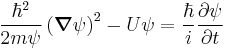
which is a nonlinear variant of the Schrödinger equation.
Conversely, starting with the Schrödinger equation and our Ansatz for , we arrive at[4]
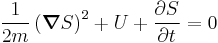
The classical limit ( ) of the Schrödinger equation above becomes identical to the following variant of the Hamilton–Jacobi equation,
The Hamilton–Jacobi equation in the gravitational field
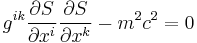
where  are the contravariant coordinates of the metric tensor, m is the rest mass of the particle and c is the speed of light.
See also
- Hamilton's principal function
- Canonical transformation
- Constant of motion
- Hamiltonian vector field
- Hamilton–Jacobi–Bellman equation in control theory
- WKB approximation
- William Rowan Hamilton
- Carl Gustav Jacob Jacobi
- Action-angle coordinates
References
- ^ Goldstein, pp. 484–492, particularly the discussion beginning in the last paragraph of page 491.
- ^ Sakurai, pp. 103–107.
- ^ Herbert Goldstein, Classical Mechanics, 2nd ed. (Reading, Mass.: Addison-Wesley, 1981), p. 440.
- ^ Goldstein, pp. 490–491.
Further reading
- Hamilton, W. (1833). "On a General Method of Expressing the Paths of Light, and of the Planets, by the Coefficients of a Characteristic Function". Dublin University Review: 795–826.
- Hamilton, W. (1834). "On the Application to Dynamics of a General Mathematical Method previously Applied to Optics". British Association Report: 513–518.
- Goldstein, H. (2002). Classical Mechanics. Addison Wesley. ISBN 0201657023.
- Fetter, A. & Walecka, J. (2003). Theoretical Mechanics of Particles and Continua. Dover Books. ISBN 0486432610.
- Landau, L. D.; Lifshitz, L. M. (1975). Mechanics. Amsterdam: Elsevier.
- Sakurai, J. J. (1985). Modern Quantum Mechanics. Benjamin/Cummings Publishing. ISBN 0805375015.